If you're dealing with datasets so massive they laugh at the memory capacity of a single machine, you've probably heard of Apache Spark. And if you’re a Python developer, you’re in luck. The go-to method for wrangling this kind of big data is PySpark—the beautiful marriage of Python's simplicity and Spark's distributed computing muscle.
It lets you take on enormous data processing tasks with a speed and efficiency that feels like a superpower.
Why PySpark Became the Key to Big Data
To really get why PySpark is such a big deal, you have to remember what life was like before it. Big data processing was a slow, agonizing affair. Most systems were shackled to disk-based operations, which just couldn't keep up as data volumes exploded. We needed a better, faster way to get insights from terabytes of information without waiting hours—or even days—for a single job to finish.
That’s the problem Apache Spark was built to solve. Born at UC Berkeley's AMPLab in 2009, it flipped the script by focusing on in-memory computing. Instead of constantly shuffling data back and forth from slow hard drives, Spark does its work in RAM. This simple change makes it up to 100 times faster for certain tasks.
PySpark is simply the Python API for this powerhouse engine, making all that speed and scale accessible to the millions of developers who already know and love Python. It’s the best of both worlds. You can see a great comparative analysis of how it stacks up against other tools.
What’s Under the Hood? The Core Strengths of Spark
So, what makes Spark so special? It's not just one thing, but a combination of smart architectural decisions designed for speed, scale, and reliability.
Before we jump into code, it helps to get a handle on the fundamental concepts that make Spark tick. These are the building blocks of every PySpark application.
Key Apache Spark Concepts at a Glance
| Concept | Description | Role in PySpark |
|---|---|---|
| Cluster | A group of computers (nodes) that work together as a single system. | The hardware foundation. Spark distributes data and computations across the cluster. |
| Driver | The main process that runs your main() function and creates the SparkContext. | It's the "brain" of your PySpark application, coordinating tasks across the cluster. |
| Executor | Processes that run on worker nodes to execute the tasks assigned by the driver. | These are the "hands" doing the actual work, like reading data and running calculations. |
| RDD | Resilient Distributed Dataset. The original, low-level data structure in Spark. | An immutable, fault-tolerant collection of objects partitioned across the cluster. |
| DataFrame | A distributed collection of data organized into named columns, like a table. | The primary, high-level API you'll use. It's easier to work with than RDDs and highly optimized. |
| SparkSession | The single entry point to all Spark functionality. | You use it to create DataFrames, register UDFs, and execute SQL queries. |
Understanding these pieces is the first step. The driver directs the work, the executors do the heavy lifting, and the SparkSession is how you command them all.
Now, let's look at the principles that make this system work so well.
-
Speed Through In-Memory Processing: By holding data in memory between steps, Spark dodges the massive bottleneck of writing to disk. This is a game-changer for iterative algorithms, like those in machine learning, and for interactive, exploratory analysis.
-
Distributed by Design: Spark was built from the ground up to be distributed. It automatically slices up huge jobs into smaller tasks and spreads them across a cluster of machines. This horizontal scaling means if your data grows, you just add more computers to handle it. Simple as that.
-
Fault Tolerance with RDDs: The foundation of Spark is a concept called the Resilient Distributed Dataset (RDD). You can think of an RDD as a recipe for a dataset that’s spread across your cluster. If one of your computers dies in the middle of a calculation, Spark can use that recipe to automatically rebuild the lost piece of data. Your job just keeps running.
The big picture: It's this fusion of in-memory speed and a distributed, fault-tolerant architecture that lets PySpark handle petabyte-scale datasets without breaking a sweat.
Python Meets Big Data Power
The real magic happens when Spark's raw power is paired with Python's elegance. PySpark acts as the perfect translator, letting you write clean, readable Python code that Spark executes across a massive cluster.
You get the rich ecosystem of Python libraries for things like data cleaning and visualization, but with the computational engine of a world-class distributed system.
For instance, a data scientist can use a library they already know, like Pandas, to explore a small sample of data. Once they’ve figured out their logic, they can apply the exact same steps to a gargantuan dataset using PySpark’s DataFrame API, which was intentionally designed to feel familiar to Pandas users.
This powerful synergy is why learning Apache Spark in Python has become a non-negotiable skill for anyone serious about solving today's data challenges.
Getting Your PySpark Environment Ready
Before you can start wrangling massive datasets with Apache Spark in Python, you first need to get your local environment squared away. You don't need to jump straight into a complex, multi-node cluster to get started. In fact, a local installation on your own machine is the perfect sandbox for learning the ropes.
The good news? The Python ecosystem makes this setup incredibly straightforward.
The simplest path forward is using pip, Python's trusty package installer. This method is fantastic because it bundles everything you need to run Spark locally, so you don't have to deal with a separate, manual download of the Spark framework itself. It's the fast track to getting your hands dirty with code.
Just pop open= your terminal or command prompt and run this one command:
pip install pyspark
That single line fetches the PySpark library and all its dependencies. Crucially, it also includes a local Spark instance, which is super convenient for development and testing. Once that finishes up, you're ready for the most important step: firing up a SparkSession.
Launching Your First SparkSession
Think of the SparkSession as your gateway to the entire Spark world. It's the main entry point for all Spark functionality, and you absolutely have to create an instance of it before you can do anything else. This one object is responsible for managing your Spark application, from configuring resources to coordinating the execution of your data processing jobs.
Creating a SparkSession is a small but vital piece of boilerplate code that will kick off nearly every PySpark script you write. Here’s the standard way to do it:
from pyspark.sql import SparkSession

# Create a SparkSession
spark = SparkSession.builder \
    .appName("FirstPySparkApp") \
    .getOrCreate()

# Print the SparkSession object to confirm it's running
print(spark)
So, what's happening here? The .appName() method just gives your application a friendly name, which is a big help when you're monitoring jobs in the Spark UI. The .getOrCreate() method is pretty smart—it either spins up a new SparkSession or, if one is already running, it just grabs that existing one. This is a neat trick to prevent you from accidentally running multiple= Spark contexts.
Verifying Your Installation
With your SparkSession initialized, you should run a quick check to make sure everything is humming along nicely. A classic "hello world" for PySpark is to create a simple DataFrame and show its contents. It’s an instant confirmation that your environment is good to go.

This little snippet creates a DataFrame from a small, in-memory list of data and then uses the .show() method to print it right to your console.
# Create a sample list of data
data = [("Alice", 1), ("Bob", 2), ("Charlie", 3)]
columns = ["name", "id"]

# Create a DataFrame from the sample data
df = spark.createDataFrame(data, columns)

# Display the DataFrame
df.show()

# Stop the SparkSession to release resources
spark.stop()
If you see a neatly formatted table with "name" and "id" columns printed to your console, congratulations! Your local Apache Spark in Python environment is up and running. Managing data structures like this is a core skill, and if you work in cloud environments, you might find our guide on how Databricks simplifies creating tables useful, as it builds directly on these foundational concepts.
Key Takeaway: The
SparkSessionis the heart of your application. Always initialize it at the beginning of your script and, just as importantly, remember to callspark.stop()at the end. This gracefully shuts down the session and frees up system resources—a critical best practice that prevents memory leaks and ensures your application terminates cleanly.
Working with DataFrames and Spark SQL
Once your environment is up and running, it's time to get your hands dirty with the core of Apache Spark in Python: the DataFrame API.
So, what exactly is a DataFrame? The best way to think of it is as a supercharged, distributed table. It has the familiar structure of a spreadsheet or a SQL table, but with one massive advantage—it's spread across many computers. This design is what lets it chew through datasets of almost any size. This is where the real data crunching begins.
To make this tangible, let's walk through a classic e-commerce scenario. We've got a CSV file, sales_data.csv, containing columns like order_id, product_name, category, price, and purchase_date. Our mission is to turn this raw data into some real business insights.
Loading and Inspecting Your Data
First things first, we need to get our data into Spark. Luckily, PySpark makes reading common formats like CSV, Parquet, or JSON incredibly straightforward. Let's load up our sales data.
from pyspark.sql import SparkSession

# Always start by initializing a SparkSession
spark = SparkSession.builder.appName("SalesAnalysis").getOrCreate()

# Read the CSV file into a DataFrame
sales_df = spark.read.csv("sales_data.csv", header=True, inferSchema=True)

# A quick sanity check to see the first few rows
sales_df.show(5)

# And let's inspect the data types Spark assigned
sales_df.printSchema()
A couple of things to note here. header=True tells Spark that the first line in our file is the column names. The inferSchema=True option is a real time-saver during development; it has Spark scan the data and take its best guess at the data type for each column. While great for quick analysis, it's a good practice in production code to define the schema yourself for better performance and to avoid any surprises.
Selecting and Filtering Data
With our data loaded, we can start asking questions. The two most fundamental operations you'll use constantly are selecting columns and filtering rows. These are the absolute bread and butter of any data transformation.
The select() method lets you cherry-pick the columns you care about, which is perfect for creating a smaller, more focused view of your dataset.
# Just grab the product name and its price
product_prices_df = sales_df.select("product_name", "price")
product_prices_df.show(5)
Next up is filter() (which also has an alias, where()). This is how you trim your dataset down to rows that match a specific condition. For instance, let's isolate all the sales from the "Electronics" category.
# Keep only the rows where the category is 'Electronics'
electronics_sales_df = sales_df.filter(sales_df.category == "Electronics")
electronics_sales_df.show(5)
The real power comes from chaining these operations together. You can build up a sequence of clean, readable transformations, which is a core philosophy of the DataFrame API.
Performing Aggregations with GroupBy
Aggregations are where you start to summarize your data and uncover high-level insights. Your go-to tool for this is the groupBy() method. It collapses your DataFrame by one or more columns, which then lets you run aggregate functions like count(), sum(), avg(), min(), or max() on each group.
Let's figure out the total revenue generated by each product category.
from pyspark.sql.functions import sum

# Group by the category column, then sum up the price for each group
category_revenue_df = sales_df.groupBy("category").agg(sum("price").alias("total_revenue"))

# Show the results, with the highest revenue categories at the top
category_revenue_df.orderBy("total_revenue", ascending=False).show()
The .agg() function is where you define what calculation to perform on the groups. Notice the .alias() method? We use it here to give our new column a clean name, total_revenue. This simple query instantly tells us which of our product categories are bringing in the most money.
A Pro Tip From Experience: Always use
alias()to rename your aggregated columns. If you don't, Spark gives them default names likesum(price), which are awkward to reference in later steps. Keeping your column names clean makes your code so much easier to read and maintain.
Harnessing the Power of Spark SQL
One of the absolute best features of using Apache Spark in Python is that you don't have to leave your SQL skills at the door. Spark SQL lets you run standard SQL queries directly against your DataFrames. It's an incredibly powerful feature that lets you express complex logic in a language many data folks already know and love.
To get started, you just need to register your DataFrame as a temporary "view." This doesn't actually copy or move any data; it simply gives the Spark SQL engine a name it can use in a query.
# Create a temporary view that we can query with SQL
sales_df.createOrReplaceTempView("sales_table")

# Now, we can write a good old-fashioned SQL query
high_value_electronics_sql = """
    SELECT product_name, price
    FROM sales_table
    WHERE category = 'Electronics' AND price > 500
    ORDER BY price DESC
"""

high_value_df = spark.sql(high_value_electronics_sql)
high_value_df.show()
The result of spark.sql() is just another DataFrame. You can then continue to work with it using the DataFrame API, or even register it as another view for more SQL queries. This seamless blend of the two APIs gives you amazing flexibility.
Sometimes, a tricky bit of string manipulation or conditional logic is just plain easier to write in SQL. For more advanced text operations, you might even find yourself exploring techniques for Python fuzzy string matching, which can be integrated into Spark via user-defined functions. This hybrid approach lets you pick the best tool for each specific task in your pipeline.
Building a Real-World PySpark Application
Alright, we've covered the core PySpark operations. Now it’s time to put it all together and solve a real problem. Knowing the syntax is one thing, but applying it to a messy, real-world scenario is how you really start thinking like a data engineer.
Let's walk through a classic business request: analyzing raw customer reviews to figure out which product features people talk about the most. We have a pile of unstructured text feedback, and our job is to turn it into a clean, summarized report that a product manager can actually use.
The Scene: Messy Data, Clear Goal
We're starting with a simple CSV file, reviews.csv, which has just two columns: review_id and review_text. The text itself is a free-for-all—mixed casing, random punctuation, and full of common "stop words" (like 'a', 'is', 'the') that don't tell us much.
Our plan is to build a pipeline that will:
- Load the raw text into a PySpark DataFrame.
- Clean it up by making everything lowercase and stripping out punctuation.
- Tokenize the reviews, which just means splitting them into individual words.
- Filter out all those useless stop words.
- Count how many times each meaningful word appears.
- Save the final counts into a new CSV for the product team.
This process takes a stream of chaotic customer feedback and turns it into a structured, actionable list of key terms.
Kicking Off the Transformation Pipeline
First things first, we need to initialize a SparkSession and get our data loaded. This is the standard opening for pretty much any PySpark job you'll ever write.
from pyspark.sql import SparkSession
from pyspark.sql.functions import lower, regexp_replace, split, explode, col
from pyspark.ml.feature import StopWordsRemover

# Get our SparkSession going
spark = SparkSession.builder.appName("ReviewAnalysis").getOrCreate()

# Load the raw data from the CSV
reviews_df = spark.read.csv("reviews.csv", header=True, inferSchema=True)
With the DataFrame ready, our first real transformation is to clean the text. We can chain a couple of functions here: lower() to standardize the case and regexp_replace() to yank out any character that isn't a letter or a space.
# Clean up the review text
cleaned_df = reviews_df.withColumn("cleaned_text",
    lower(col("review_text"))
).withColumn("cleaned_text",
    regexp_replace(col("cleaned_text"), "[^a-z\\s]", "")
)
Just like that, our DataFrame now has a cleaned_text column with a much tidier version of the original reviews.
Extracting Keywords and Counting Frequencies
Now for the fun part. We'll use split() to tokenize the text in our new column, which creates an array of words for each review. Then, we bring in explode(), a seriously powerful function that takes each array and creates a new row for every single word in it.
# Turn sentences into lists of words, then explode them into rows
words_df = cleaned_df.withColumn("words", split(col("cleaned_text"), "\\s+"))
exploded_df = words_df.select("review_id", explode(col("words")).alias("word"))
Before we can count anything, we need to get rid of the noise. PySpark’s machine learning library has a StopWordsRemover that's perfect for this.
# Filter out common stop words like 'the', 'a', 'is'
remover = StopWordsRemover(inputCol="word", outputCol="filtered_word")
filtered_words_df = remover.transform(exploded_df)
Finally, a simple groupBy() and count() gives us the frequency of every remaining word.
# Count the occurrences of each word
word_counts_df = filtered_words_df.groupBy("filtered_word").count()

# Show the most talked-about terms
word_counts_df.orderBy(col("count").desc()).show()
The output is a clean, two-column DataFrame that gives us immediate insight into what customers are actually talking about. This entire workflow is a great example of how you can use Apache Spark in Python for basic natural language processing.
Delivering the Final Insights
The last step is to get our results out of Spark and into a format someone can use. Writing the DataFrame to a CSV or Parquet file makes it easy to share with other teams or plug into a visualization tool.
# Save the results to a single, clean CSV file
word_counts_df.orderBy(col("count").desc()).coalesce(1).write.csv("top_features.csv", header=True)
A Quick Note on
coalesce(1): Spark is a distributed system, so by default, it writes output in multiple= parts (one for each data partition). Using.coalesce(1)tells Spark to gather all the data onto a single worker before writing, giving you one nice output file. It’s perfect for small result sets like this one, but be careful using it with massive datasets—it can create a bottleneck.
Seeing how data moves from a source through various transformations is crucial. This infographic gives a great visual of a common workflow that combines the DataFrame API with Spark SQL.
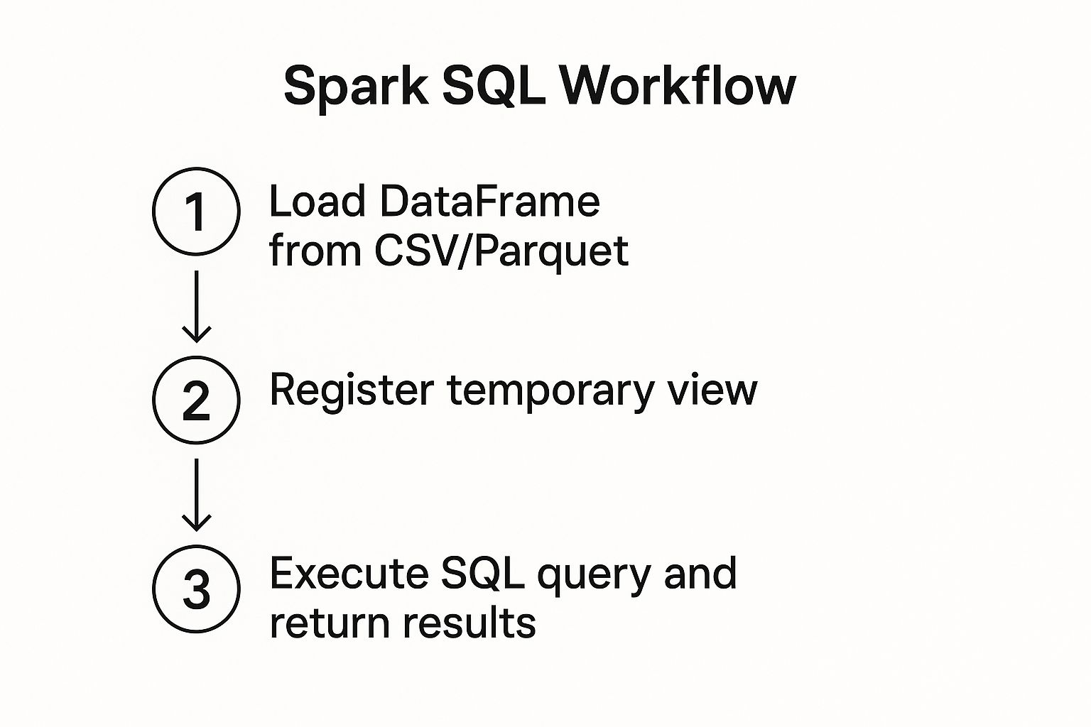
As the diagram shows, you can register a DataFrame as a temporary view. This lets you switch back and forth between PySpark's functions and standard SQL queries, giving you a ton of flexibility to get the job done.
This whole process—from messy text to a ranked list of product features—shows off the real power of PySpark. Each transformation builds logically on the last, turning otherwise useless unstructured data into a real business asset. If you're curious about how models process this type of information, you can dig deeper into what is model context protocol in our other guide.
Tuning Performance with the Spark UI
Getting your PySpark code to work is one thing. Getting it to run fast is what separates a good data engineer from a great one. An unoptimized job can absolutely torch your cloud budget, eating up compute time and money.
The secret to making your jobs fly is understanding what’s happening under the hood. For that, your best friend is the Spark UI.
The Spark UI isn't just a simple dashboard; it’s a powerful diagnostic tool that gives you an x-ray view into your application's execution. It visualizes everything from resource usage to the exact execution plan, making it perfect for hunting down bottlenecks. By default, it runs on port 4040 on your driver node, and learning to read it is a non-negotiable skill for anyone serious about writing scalable Spark jobs.
Navigating the Job Execution Graph
Every time you call an action like .show() or .write(), Spark kicks off a job. Inside the Spark UI, you'll see this job broken down into stages, which are then made up of individual tasks. This whole workflow is visualized as a Directed Acyclic Graph (DAG), which is basically a flowchart of the operations Spark plans to execute.
Learning to read this graph is where the magic happens. You can see precisely how Spark is reading data, what transformations it's applying, and—most importantly—where it's shuffling data across the network.
A "shuffle" is a notoriously expensive operation where Spark has to physically move data between different executors. When you see a wide, complex stage in your DAG, that's often a dead giveaway for a shuffle. It's the first place I look when a job is running slow.
Key Optimization Techniques
Before we get lost in the UI, there are a couple of straightforward techniques that can give you some quick wins on performance: caching and smart partitioning.
-
Caching with
cache()orpersist(): If you're using the same DataFrame multiple= times, Spark will recompute it from scratch every single time by default. That's incredibly wasteful. By callingdf.cache(), you’re telling Spark, "Hey, calculate this once and then hang onto it in memory." Any subsequent actions will pull from the in-memory cache, which is orders of magnitude faster.# An example of caching to speed up multiple actions filtered_df = sales_df.filter(sales_df.price > 100) filtered_df.cache() # Store this filtered DataFrame in memory # Action 1: Count high-value items print(f"Number of high-value items: {filtered_df.count()}") # Action 2: Show the top 5 filtered_df.show(5) # Without .cache(), the filtering would happen twice! -
Smart Partitioning: Spark achieves parallelism by splitting your data into partitions. Too few partitions, and you’re leaving cluster resources on the table. Too many, and the overhead of managing them all will drag your job down. Using
repartition()orcoalesce()to get the partition count just right for your data size and cluster is a game-changer.# Example of repartitioning before a join # Assume we have another DataFrame, customer_df, to join with # Repartitioning both on the join key can speed things up partitioned_sales = sales_df.repartition("customer_id") partitioned_customers = customer_df.repartition("customer_id") joined_df = partitioned_sales.join(partitioned_customers, "customer_id")
Be careful not to get too
cache()-happy. A common mistake is caching everything, which can quickly exhaust your executor memory. This forces Spark to spill data to disk or, even worse, crash your job with out-of-memory errors. Only cache DataFrames that are genuinely expensive to compute and are used more than once.
Spotting Bottlenecks in the Spark UI
When I'm troubleshooting, the Stages tab is my first stop. It gives you a high-level summary of every stage, including its duration, the number of tasks, and how much data was read or shuffled.
If one stage is taking way longer than the others, you've found your bottleneck. Click into it for a task-level breakdown. Do you see a few tasks taking significantly longer than the average? That's a classic case of data skew, where some partitions have way more data than others. The fix is often to repartition your data with a key that ensures a more even distribution.
For a quick reference on where to start with optimizations, here's a table of common techniques I use.
Common PySpark Optimization Techniques
| Technique | What It Does | Best Use Case |
|---|---|---|
Caching (.cache()) | Stores an intermediate DataFrame in memory to avoid re-computation. | When a DataFrame is used multiple= times in subsequent transformations or actions. |
Repartitioning (.repartition()) | Increases or decreases the number of partitions, involving a full data shuffle. | Fixing data skew or preparing a DataFrame for a join on a specific key. |
Coalescing (.coalesce()) | Reduces the number of partitions efficiently without a full shuffle. | When you've filtered a large dataset and want to reduce partitions before writing to disk. |
| Broadcasting | Sends a small DataFrame to every executor node to avoid a shuffle during a join. | Joining a very large DataFrame with a very small one (e.g., a lookup table). |
| Predicate Pushdown | Pushes filter() operations down to the data source level to read less data. | Filtering data from Parquet, ORC, or JDBC sources as early as possible. |
| Salting | Adds a random prefix to join keys to distribute skewed data more evenly across partitions. | When a few keys are responsible for a large portion of the data in a join. |
Mastering these strategies will help you write much more efficient and robust PySpark jobs.
The demand for these skills is only growing. The future of Spark is all about making these massive-scale operations more efficient. Projections for 2025 show Spark’s expanding footprint in global markets. For instance, the financial sector is expected to see 45% of organizations adopt Spark for real-time fraud detection, and 70% of e-commerce platforms are predicted to use it for customer analytics. You can read more about these projections for big data frameworks on moldstud.com.
By combining smart coding practices with a little detective work in the Spark UI, you can turn a slow, clunky job into a lean, efficient data processing machine.
Common PySpark Questions Answered
As you get your hands dirty with PySpark, you'll quickly run into a few common questions. These are the kinds of things that trip up newcomers and even seasoned pros when designing new data pipelines. Let's clear up some of that confusion.

Think of this section as your quick-reference FAQ for the big questions that can make or break your architectural decisions.
PySpark Versus Pandas What Is the Difference
This is easily the most common question I hear. While the DataFrame APIs for both libraries can look suspiciously similar at first glance, they are built for fundamentally different worlds.
Pandas is the undisputed champion for single-machine data analysis. If your dataset can comfortably fit into your computer's RAM, Pandas is your go-to. It's incredibly fast and intuitive for that scale.
PySpark, on the other hand, was born for distributed computing. It’s designed to process data in parallel across a whole cluster of machines. When your data is too big for one computer, PySpark shines.
Key Takeaway: Think of it this way: Pandas is for kilobytes or megabytes. PySpark is for gigabytes, terabytes, or even petabytes. Choose Pandas for smaller, single-node tasks and PySpark when you're wading into big data.
When Should I Use an RDD Instead of a DataFrame
Another frequent point of confusion is when to reach for the older Resilient Distributed Dataset (RDD) API instead of the modern DataFrame. The guidance here is pretty straightforward.
For 95% of use cases, you should stick with DataFrames. Period.
The DataFrame API is built on top of the Spark SQL engine, which gives you access to the powerful Catalyst Optimizer. This engine analyzes your code and figures out the most efficient way to execute it, giving you huge performance boosts automatically. You just don't get that with RDDs.
So when would you use an RDD? Only in very specific scenarios. Maybe you're working with totally unstructured data like raw server logs, or you need extremely fine-grained, manual control over how your data is partitioned and processed. Otherwise, DataFrames are the smarter, faster choice.
How Can I Handle Errors in a PySpark Job
Building robust error handling is what separates a prototype from a production-ready job. A solid strategy involves a few layers.
At a high level, wrap your driver program's logic in try-except blocks. This is your first line of defense for catching major exceptions that could crash the entire job.
# A simple try-finally block to ensure Spark stops
try:
    df = spark.read.csv("non_existent_file.csv", header=True)
    df.show()
except Exception as e:
    print(f"An error occurred: {e}")
finally:
    # This block will run whether an error occurred or not
    spark.stop()
    print("SparkSession has been stopped.")
Within your transformations, focus on data quality. This means proactively checking for and filtering out nulls, using when() and otherwise() for conditional logic, and—my personal favorite—routing malformed records to a separate "bad records" path. This lets the main job complete while you investigate the bad data later.
Finally, get comfortable with the Spark UI. It's your best friend for diagnosing failed tasks, spotting performance bottlenecks, and identifying data skew that might be causing silent errors.
At FindMCPServers, we're focused on advancing AI capabilities. Explore our platform to discover MCP servers and tools that can connect your LLMs to external data sources, simplifying complex integrations. Learn more at https://www.findmcpservers.com.